■ 텐써플로우 다층 신경망 구성
*underfitting 을 막을 수 있는 방법
1. 가중치 초기화
2. 배치 정규화
*Overfitting 을 막을 수 있는 방법
1. 드롭아웃
■ 텐써플로우에서 가중치 초기화 하는 방법
1. Xavier ---> 1 / √n
2. He -------> √2 / n
############################################
# 가중치 초기화 방법
# W = tf.Variable(tf.random_uniform([784,10], -1, 1))
# [784,10] 형상을 가진 -1~1 사이의 균등분포 어레이
# W = tf.get_variable(name="W", shape=[784, 10], initializer=tf.contrib.layers.xavier_initializer()) # xavier 초기값
# W = tf.get_variable(name='W', shape=[784, 10], initializer=tf.contrib.layers.variance_scaling_initializer()) # he 초기값
# he 는 he 라고 안나옴
# b = tf.Variable(tf.zeros([10]))
############################################
문제36. 가중치값을 He 로 바꾸시오
x = tf.placeholder("float",[None,784])
W = tf.get_variable(name='W', shape=[784, 10], initializer=tf.contrib.layers.variance_scaling_initializer())
b = tf.Variable(tf.ones([10]))
y = tf.matmul(x,W) + b
y_hat = tf.nn.softmax(y)
y_predict = tf.argmax(y_hat, axis = 1)
*텐써플로우에서 가중치 초기화 할 때 주의 사항
주피터 노트북과 스파이더는 오류가 나므로 tf.reset_default_graph()
를 맨 위에다가 적어줘야한다.
텐써 플로우는 그래프를 메모리에 올려서 실행하게 되는데
파이참은 코드를 매번 실행할 때 마다 메모리를 지워주는데
스파이더나 쥬피터는 대화형이라서 실행할 때 마다 메모리에
그래프가 누적이 되어서 맨위에 tf.reset_default_graph() 를 적어줘야 한다.
문제37. 러닝 레이트를 0.005 로 하고 학습시키고 정확도를 확인하시오
import tensorflow as tf
tf.reset_default_graph()
from tensorflow.examples.tutorials.mnist import input_data
mnist = input_data.read_data_sets('MNIST_data/', one_hot = True)
# 계층 생성
x = tf.placeholder("float",[None,784])
W = tf.get_variable(name='W', shape=[784, 10], initializer=tf.contrib.layers.variance_scaling_initializer())
b = tf.Variable(tf.ones([10]))
y = tf.matmul(x,W) + b
y_hat = tf.nn.softmax(y)
y_predict = tf.argmax(y_hat, axis = 1)
# 라벨을 저장하기 위한 변수 생성
y_onehot = tf.placeholder("float",[None,10])
y_label = tf.argmax(y_onehot, axis = 1)
# 정확도를 출력하기 위한 변수 생성
correct_prediction = tf.equal(y_predict, y_label)
acc = tf.reduce_mean(tf.cast(correct_prediction,"float"))
# 교차 엔트로피 오차 함수
loss = -tf.reduce_sum(y_onehot * tf.log(y_hat), axis = 1)
# SGD 경사 감소법
# optimizer = tf.train.GradientDescentOptimizer(learning_rate=0.05)
# Adam 경사 감소법
optimizer = tf.train.AdamOptimizer(learning_rate=0.005)
# 학습 오퍼레이션 정의
Train = optimizer.minimize(loss)
# 변수 초기화
init = tf.global_variables_initializer()
with tf.Session() as sess:
sess.run(init)
for i in range(10000):
batch_xs, batch_ys = mnist.train.next_batch(100)
sess.run(Train, feed_dict={x : batch_xs, y_onehot : batch_ys})
if i % 600 == 0:
print(i / 600 + 1,'ecpo acc:', sess.run(acc, feed_dict={x:batch_xs, y_onehot: batch_ys}))
1.0 ecpo acc: 0.29
2.0 ecpo acc: 0.91
3.0 ecpo acc: 0.93
4.0 ecpo acc: 0.96
5.0 ecpo acc: 0.97
6.0 ecpo acc: 0.91
7.0 ecpo acc: 0.98
8.0 ecpo acc: 0.93
9.0 ecpo acc: 0.96
10.0 ecpo acc: 0.94
11.0 ecpo acc: 0.93
12.0 ecpo acc: 0.92
13.0 ecpo acc: 0.91
14.0 ecpo acc: 0.96
15.0 ecpo acc: 0.93
16.0 ecpo acc: 0.95
17.0 ecpo acc: 0.06
*아직 렐루도 안썼고 해서 정확도가 떨어진다.
문제38. 위의 단층 신경망을 다층(2층) 신경망으로 변환해서 돌리시오
0층 ---> 1층 ------------------->0층 ---> 1층 ---> 2층
단층 다층
# 입력층
# 은닉 1층
# 출력 2층
import tensorflow as tf
tf.reset_default_graph()
from tensorflow.examples.tutorials.mnist import input_data
mnist = input_data.read_data_sets('MNIST_data/', one_hot = True)
# 계층 생성
# 입력층
x = tf.placeholder("float",[None,784])
# 은닉 1층
W1 = tf.get_variable(name='W1', shape=[784, 50], initializer=tf.contrib.layers.variance_scaling_initializer())
b1 = tf.Variable(tf.ones([50]))
y1 = tf.matmul(x,W1) + b1
y_relu = tf.nn.relu(y1) # relu 활성화 함수 사용, 은닉2층의 입력값으로 사용 !!
# 은닉 2층
W2 = tf.get_variable(name='W2', shape=[50, 10], initializer=tf.contrib.layers.variance_scaling_initializer())
b2 = tf.Variable(tf.ones([10]))
y2 = tf.matmul(y_relu,W2) + b2
y_hat = tf.nn.softmax(y2)
# 예측값 출력
y_predict = tf.argmax(y_hat, axis = 1)
# 라벨을 저장하기 위한 변수 생성
y_onehot = tf.placeholder("float",[None,10])
y_label = tf.argmax(y_onehot, axis = 1)
# 정확도를 출력하기 위한 변수 생성
correct_prediction = tf.equal(y_predict, y_label)
acc = tf.reduce_mean(tf.cast(correct_prediction,"float"))
# 교차 엔트로피 오차 함수
loss = -tf.reduce_sum(y_onehot * tf.log(y_hat), axis = 1)
# SGD 경사 감소법
# optimizer = tf.train.GradientDescentOptimizer(learning_rate=0.05)
# Adam 경사 감소법
optimizer = tf.train.AdamOptimizer(learning_rate=0.001)
#학습률 0.05 로 하니까 난리남
# 학습 오퍼레이션 정의
Train = optimizer.minimize(loss)
# 변수 초기화
init = tf.global_variables_initializer()
with tf.Session() as sess:
sess.run(init)
for i in range(10000):
batch_xs, batch_ys = mnist.train.next_batch(100)
sess.run(Train, feed_dict={x : batch_xs, y_onehot : batch_ys})
if i % 600 == 0:
print(i / 600 + 1,'ecpo acc:', sess.run(acc, feed_dict={x:batch_xs, y_onehot: batch_ys}))
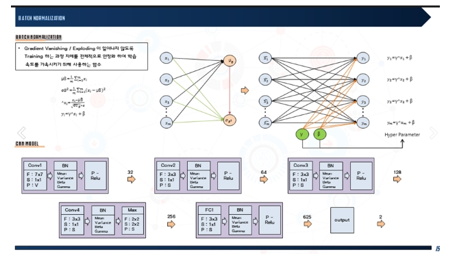
■ 텐써플로우로 배치 정규화 구현
배치정규화?
신경망 학습 시 가중치값의 데이터가 골고루 분산 될 수 있게
하는 것을 강제하는 장치
구현코드?
batch_z1 = tf.contrib.layers.batch_norm(z1, True)
가중치의 합 내적-->배치정규화-->relu 함수
문제39. 문제 38번에서 완성한 2층 신경망에 배치정규화 코드를 추가해서
돌리고 정확도를 확인하시오
# 입력층
x = tf.placeholder("float",[None,784])
# 은닉 1층
W1 = tf.get_variable(name='W1', shape=[784, 50], initializer=tf.contrib.layers.variance_scaling_initializer())
b1 = tf.Variable(tf.ones([50]))
y1 = tf.matmul(x,W1) + b1
#print(y1.shape) (?, 50)
batch_y1 = tf.contrib.layers.batch_norm(y1, True) #내적시킨값을 분산시킨다
y_relu = tf.nn.relu(batch_y1) # relu 활성화 함수 사용, 은닉2층의 입력값으로 사용 !!
# 은닉 2층
W2 = tf.get_variable(name='W2', shape=[50, 10], initializer=tf.contrib.layers.variance_scaling_initializer())
b2 = tf.Variable(tf.ones([10]))
y2 = tf.matmul(y_relu,W2) + b2
y_hat = tf.nn.softmax(y2)
1.0 ecpo acc: 0.21
2.0 ecpo acc: 0.95
3.0 ecpo acc: 0.92
4.0 ecpo acc: 0.99
5.0 ecpo acc: 0.97
6.0 ecpo acc: 0.99
7.0 ecpo acc: 0.97
8.0 ecpo acc: 0.99
9.0 ecpo acc: 0.95
10.0 ecpo acc: 0.99
11.0 ecpo acc: 0.97
12.0 ecpo acc: 1.0
13.0 ecpo acc: 1.0
14.0 ecpo acc: 1.0
15.0 ecpo acc: 1.0
16.0 ecpo acc: 0.99
17.0 ecpo acc: 1.0
■ 훈련하는 신경망에 테스트를 하는 코드를 추가
문제40. 지금 현재까지의 코드는 신경망을 훈련만 시키는 코드 였는데
테스트 데이터도 신경망에 입력해서 오버피팅이 발생하는지
확인할 수 있도록 훈련 데이터의 정확도와 테스트 데이터의 정확도를
같이 출력 할 수 있도록 코드를 작성하시오
with tf.Session() as sess:
sess.run(init)
for i in range(10000):
train_xs, train_ys = mnist.train.next_batch(100)
test_xs, test_ys = mnist.test.next_batch(100)
sess.run(Train, feed_dict={x : train_xs, y_onehot : train_ys})
if i %600 == 0:
print(i/600+1, 'epoc train acc:', sess.run(acc, feed_dict={x:train_xs, y_onehot:train_ys}))
print(i/600+1, 'epoc test acc :', sess.run(acc, feed_dict={x:test_xs, y_onehot:test_ys}))
print('=============================================')
1.0 epoc train acc: 0.11
1.0 epoc test acc : 0.1
=============================================
2.0 epoc train acc: 0.97
2.0 epoc test acc : 0.96
=============================================
3.0 epoc train acc: 0.96
3.0 epoc test acc : 0.93
=============================================
4.0 epoc train acc: 0.91
4.0 epoc test acc : 0.95
=============================================
5.0 epoc train acc: 0.97
5.0 epoc test acc : 0.96
=============================================
6.0 epoc train acc: 0.98
6.0 epoc test acc : 1.0
=============================================
7.0 epoc train acc: 0.99
7.0 epoc test acc : 0.93
=============================================
8.0 epoc train acc: 0.98
8.0 epoc test acc : 0.97
=============================================
9.0 epoc train acc: 0.99
9.0 epoc test acc : 0.94
=============================================
10.0 epoc train acc: 0.99
10.0 epoc test acc : 0.96
=============================================
11.0 epoc train acc: 1.0
11.0 epoc test acc : 0.99
=============================================
12.0 epoc train acc: 0.99
12.0 epoc test acc : 0.98
=============================================
13.0 epoc train acc: 0.98
13.0 epoc test acc : 0.98
=============================================
14.0 epoc train acc: 1.0
14.0 epoc test acc : 0.98
=============================================
15.0 epoc train acc: 1.0
15.0 epoc test acc : 0.96
=============================================
16.0 epoc train acc: 0.99
16.0 epoc test acc : 0.98
=============================================
17.0 epoc train acc: 1.0
17.0 epoc test acc : 0.94
=============================================
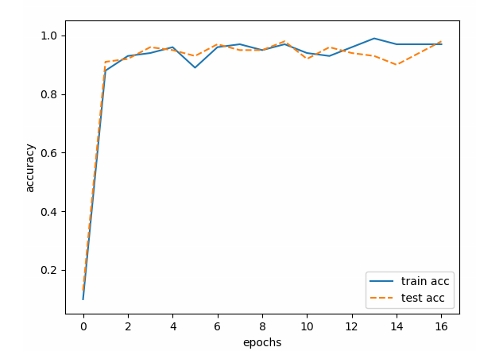
문제41. 위의 결과를 그래프로 시각화 하시오
init = tf.global_variables_initializer()
train_acc_list = []
test_acc_list = []
with tf.Session() as sess:
sess.run(init)
for i in range(10000):
train_xs, train_ys = mnist.train.next_batch(100)
test_xs, test_ys = mnist.test.next_batch(100)
sess.run(Train, feed_dict={x : train_xs, y_onehot : train_ys})
if i %600 == 0:
train_acc = sess.run(acc, feed_dict={x:train_xs, y_onehot:train_ys})
print(i/600+1, 'epoc train acc:', train_acc)
train_acc_list.append(train_acc)
test_acc = sess.run(acc, feed_dict={x:test_xs, y_onehot:test_ys})
print(i/600+1, 'epoc test acc :', test_acc)
test_acc_list.append(test_acc)
print('=============================================')
#그래프그리기
markers = {'train': 'o', 'test': 's'}
x = np.arange(len(train_acc_list))
plt.plot(x, train_acc_list, label='train acc')
plt.plot(x, test_acc_list, label='test acc', linestyle='--')
plt.xlabel("epochs")
plt.ylabel("accuracy")
plt.ylim(0, 1.0)
plt.legend(loc='lower right')
plt.show()
■ 오버피팅이 발생하지 않도록 dropout 을 적용하는 방법
문제42.(점심시간 문제)
책 132페이지를 참고해서 드롭아웃을 적용시켜서 훈련시키는데
훈련데이터는 50%, 테스트 데이터는 100% 의 노드로 하시오.
# 은닉 1층
W1 = tf.get_variable(name='W1', shape=[784, 50], initializer=tf.contrib.layers.variance_scaling_initializer())
b1 = tf.Variable(tf.ones([50]))
y1 = tf.matmul(x,W1) + b1
#print(y1.shape) (?, 50)
batch_y1 = tf.contrib.layers.batch_norm(y1, True) #내적시킨값을 분산시킨다
y_relu = tf.nn.relu(batch_y1) # relu 활성화 함수 사용, 은닉2층의 입력값으로 사용 !!
# 드롭아웃
keep_prob = tf.placeholder("float")
r1_drop = tf.nn.dropout(y_relu, keep_prob)
# 은닉 2층
W2 = tf.get_variable(name='W2', shape=[50, 10], initializer=tf.contrib.layers.variance_scaling_initializer())
b2 = tf.Variable(tf.ones([10]))
y2 = tf.matmul(r1_drop,W2) + b2
y_hat = tf.nn.softmax(y2)
:
:
with tf.Session() as sess:
sess.run(init)
for i in range(10000):
train_xs, train_ys = mnist.train.next_batch(100)
test_xs, test_ys = mnist.test.next_batch(100)
sess.run(Train, feed_dict={x : train_xs, y_onehot : train_ys, keep_prob:0.5 })
if i %600 == 0:
train_acc = sess.run(acc, feed_dict={x:train_xs, y_onehot:train_ys, keep_prob:1.0})
test_acc = sess.run(acc, feed_dict={x:test_xs, y_onehot:test_ys, keep_prob:1.0})
print(i/600+1, 'epoc train acc:', train_acc)
train_acc_list.append(train_acc)
print(i/600+1, 'epoc test acc :', test_acc)
test_acc_list.append(test_acc)
print('=============================================')
※ keep_prob 는 남기는 값.
Train 의 keep_prob:0.5 는 (50%날리고) 50% 남기겠다는 의미며,
test_acc 에 keep_prob:1.0 은 100% 다 남기겠다는 의미다.
1.0 epoc train acc: 0.1
1.0 epoc test acc : 0.13
=============================================
2.0 epoc train acc: 0.88
2.0 epoc test acc : 0.91
:
:
=============================================
17.0 epoc train acc: 0.97
17.0 epoc test acc : 0.98
=============================================
문제43. 2층 신경망 ---> 3층 신경망으로 변경하고 정확도를 확인하시오
입력층 --------> 은닉1층 --------> 은닉2층 ---------> 출력층(3층)
784 100 100 10
import tensorflow as tf
tf.reset_default_graph()
from tensorflow.examples.tutorials.mnist import input_data
import numpy as np
import matplotlib.pyplot as plt
mnist = input_data.read_data_sets('MNIST_data/', one_hot = True)
# 계층 생성
# 입력층
x = tf.placeholder("float",[None,784])
# 은닉 1층
W1 = tf.get_variable(name='W1', shape=[784, 100], initializer=tf.contrib.layers.variance_scaling_initializer())
b1 = tf.Variable(tf.ones([100]))
y1 = tf.matmul(x,W1) + b1
#print(y1.shape) (?, 50)
batch_y1 = tf.contrib.layers.batch_norm(y1, True) #내적시킨값을 분산시킨다
y_relu = tf.nn.relu(batch_y1) # relu 활성화 함수 사용, 은닉2층의 입력값으로 사용 !!
# 은닉 2층
W2 = tf.get_variable(name='W2', shape=[100, 100], initializer=tf.contrib.layers.variance_scaling_initializer())
b2 = tf.Variable(tf.ones([100]))
y2 = tf.matmul(y_relu,W2) + b2
#print(y1.shape) (?, 50)
batch_y2 = tf.contrib.layers.batch_norm(y2, True) #내적시킨값을 분산시킨다
y_relu2 = tf.nn.relu(batch_y2) # relu 활성화 함수 사용, 은닉2층의 입력값으로 사용 !!
# 드롭아웃
keep_prob = tf.placeholder("float")
r1_drop = tf.nn.dropout(y_relu2, keep_prob)
# 출력층(3층)
W3 = tf.get_variable(name='W3', shape=[100, 10], initializer=tf.contrib.layers.variance_scaling_initializer())
b3 = tf.Variable(tf.ones([10]))
y3 = tf.matmul(r1_drop,W3) + b3
y_hat = tf.nn.softmax(y3)
# 예측값 출력
y_predict = tf.argmax(y_hat, axis = 1)
# 라벨을 저장하기 위한 변수 생성
y_onehot = tf.placeholder("float",[None,10])
y_label = tf.argmax(y_onehot, axis = 1)
# 정확도를 출력하기 위한 변수 생성
correct_prediction = tf.equal(y_predict, y_label)
acc = tf.reduce_mean(tf.cast(correct_prediction,"float"))
# 교차 엔트로피 오차 함수
loss = -tf.reduce_sum(y_onehot * tf.log(y_hat), axis = 1)
# SGD 경사 감소법
# optimizer = tf.train.GradientDescentOptimizer(learning_rate=0.05)
# Adam 경사 감소법
optimizer = tf.train.AdamOptimizer(learning_rate=0.001)
# 학습 오퍼레이션 정의
Train = optimizer.minimize(loss)
# 변수 초기화
init = tf.global_variables_initializer()
train_acc_list = []
test_acc_list = []
with tf.Session() as sess:
sess.run(init)
for i in range(600*20):
train_xs, train_ys = mnist.train.next_batch(100)
test_xs, test_ys = mnist.test.next_batch(100)
sess.run(Train, feed_dict={x : train_xs, y_onehot : train_ys, keep_prob:0.5 })
if i %600 == 0:
train_acc = sess.run(acc, feed_dict={x:train_xs, y_onehot:train_ys, keep_prob:1.0})
test_acc = sess.run(acc, feed_dict={x:test_xs, y_onehot:test_ys, keep_prob:1.0})
print(i/600+1, 'epoc train acc:', train_acc)
train_acc_list.append(train_acc)
print(i/600+1, 'epoc test acc :', test_acc)
test_acc_list.append(test_acc)
print('=============================================')
#그래프그리기
markers = {'train': 'o', 'test': 's'}
x = np.arange(len(train_acc_list))
plt.plot(x, train_acc_list, label='train acc')
plt.plot(x, test_acc_list, label='test acc', linestyle='--')
plt.xlabel("epochs")
plt.ylabel("accuracy")
#plt.ylim(0, 1.0)
plt.ylim(min(min(train_acc_list),min(test_acc_list))-0.05, 1.05)
plt.legend(loc='lower right')
plt.show()
※ dropoup 을 은닉1층 뒤에 넣어주니까 훨씬 높은 정확도가 나온다.
■ 텐써플로우로 CNN 구현하기
입력층 ---> 은닉 1층 ---> 은닉 2층 ---> 은닉 3층 ---> 출력층(4층)
784 (conv-pool) 100 100 10
준하코드:
import tensorflow as tf
from tensorflow.examples.tutorials.mnist import input_data
import numpy as np
import matplotlib.pyplot as plt
tf.reset_default_graph()
mnist = input_data.read_data_sets("MNIST_data/", one_hot=True)
#입력층
x = tf.placeholder("float",[None,784])
x1 = tf.reshape(x,[-1,28,28,1])
#은닉1층
b1 = tf.Variable(tf.ones([32]))
W1 = tf.Variable(tf.random_normal([3,3,1,32],stddev = 0.01))
y1 = tf.nn.conv2d(x1, W1, strides=[1,1,1,1], padding = 'SAME')
y1 = y1 + b1
y1 = tf.nn.relu(y1)
y1 = tf.nn.max_pool(y1, ksize = [1,2,2,1], strides = [1,2,2,1], padding = 'SAME')
#은닉2층
b2 = tf.Variable(tf.ones([100]))
W2 = tf.get_variable(name='W2', shape=[14*14*32, 100], initializer=tf.contrib.layers.variance_scaling_initializer())
y2 = tf.reshape(y1, [-1, 14*14*32])
y2 = tf.matmul(y2,W2) + b2
y2 = tf.nn.relu(y2)
y2 = tf.contrib.layers.batch_norm(y2,True)
#드롭아웃
keep_prob = tf.placeholder("float")
y2_drop = tf.nn.dropout(y2, keep_prob)
# 은닉 3층
b3 = tf.Variable(tf.ones([100]))
W3 = tf.get_variable(name='W3', shape=[100, 100], initializer=tf.contrib.layers.variance_scaling_initializer())
y3 = tf.matmul(y2_drop,W3) + b3
y3 = tf.contrib.layers.batch_norm(y3,True)
#출력층
b4 = tf.Variable(tf.ones([10]))
W4 = tf.get_variable(name='W4', shape=[100, 10], initializer=tf.contrib.layers.variance_scaling_initializer()) # he 초기값
y4 = tf.matmul(y3,W4) + b4
y4 = tf.contrib.layers.batch_norm(y4,True)
y_hat = tf.nn.softmax(y4)
#예측값
y_predict = tf.argmax(y_hat,1)
# 라벨을 저장하기 위한 변수 생성
y_onehot = tf.placeholder("float",[None,10])
y_label = tf.argmax(y_onehot, axis = 1)
# 정확도를 출력하기 위한 변수 생성
correct_prediction = tf.equal(y_predict, y_label)
accuracy = tf.reduce_mean(tf.cast(correct_prediction,"float"))
# 교차 엔트로피 오차 함수
loss = -tf.reduce_sum(y_onehot * tf.log(y_hat), axis = 1)
# SGD 경사 감소법
# optimizer = tf.train.GradientDescentOptimizer(learning_rate=0.05)
# Adam 경사 감소법
optimizer = tf.train.AdamOptimizer(learning_rate=0.001)
# 학습 오퍼레이션 정의
train = optimizer.minimize(loss)
# 변수 초기화
init = tf.global_variables_initializer()
train_acc_list = []
test_acc_list = []
with tf.Session() as sess:
sess.run(init)
for j in range(20):
for i in range(600):
batch_xs, batch_ys = mnist.train.next_batch(100)
test_xs, test_ys = mnist.test.next_batch(100)
sess.run(train, feed_dict={x: batch_xs, y_onehot: batch_ys, keep_prob: 0.9})
if i == 0:
train_acc = sess.run(accuracy, feed_dict={x: batch_xs, y_onehot: batch_ys, keep_prob: 1.0})
test_acc = sess.run(accuracy, feed_dict={x: test_xs, y_onehot: test_ys, keep_prob: 1.0})
train_acc_list.append(train_acc)
test_acc_list.append(test_acc)
print('훈련', str(j + 1) + '에폭 정확도 :', train_acc)
print('테스트', str(j + 1) + '에폭 정확도 :', test_acc)
print('-----------------------------------------------')
markers = {'train': 'o', 'test': 's'}
x = np.arange(len(train_acc_list))
plt.plot()
plt.plot(x, train_acc_list, label='train acc')
plt.plot(x, test_acc_list, label='test acc', linestyle='--')
plt.xlabel("epochs")
plt.ylabel("accuracy")
plt.ylim(min(min(train_acc_list),min(test_acc_list))-0.1, 1.1)
plt.legend(loc='lower right')
plt.show()
문제44. 문제43번의 4층 신경망에 conv_pooling 층을 하나 더 추가해서
5층으로 변경을 하고 GPU에서 돌리시오
import tensorflow_gpu as tf
*fully connected = FC
입력층 ---> 은닉1층 ---> 은닉2층 ---> 은닉3층 ---> 은닉4층 ---> 출력층(5층)
(conv-pool) (conv-pool) (FC1) (FC2)
↓ ↓
필터: 32개 필터: 64개
(3x3x1) (3x3x1)
import tensorflow_gpu as tf
from tensorflow.examples.tutorials.mnist import input_data
import numpy as np
import matplotlib.pyplot as plt
tf.reset_default_graph()
mnist = input_data.read_data_sets("MNIST_data/", one_hot=True)
#입력층
x = tf.placeholder("float",[None,784])
x1 = tf.reshape(x,[-1,28,28,1])
#은닉1층
b1 = tf.Variable(tf.ones([32]))
W1 = tf.Variable(tf.random_normal([3,3,1,32],stddev = 0.01))
y1 = tf.nn.conv2d(x1, W1, strides=[1,1,1,1], padding = 'SAME')
y1 = y1 + b1
y1 = tf.nn.relu(y1)
y1 = tf.nn.max_pool(y1, ksize = [1,2,2,1], strides = [1,2,2,1], padding = 'SAME')
#은닉2층
b2 = tf.Variable(tf.ones([64]))
W2 = tf.Variable(tf.random_normal([3,3,32,64],stddev = 0.01))
y2 = tf.nn.conv2d(y1, W2, strides=[1,1,1,1], padding = 'SAME')
y2 = y2 + b2
y2 = tf.nn.relu(y2)
y2 = tf.nn.max_pool(y2, ksize = [1,2,2,1], strides = [1,2,2,1], padding = 'SAME')
#은닉3층
b3 = tf.Variable(tf.ones([100]))
W3 = tf.get_variable(name='W3', shape=[7*7*64, 100], initializer=tf.contrib.layers.variance_scaling_initializer())
y3 = tf.reshape(y2, [-1, 7*7*64])
y3 = tf.matmul(y3,W3) + b3
y3 = tf.nn.relu(y3)
y3 = tf.contrib.layers.batch_norm(y3,True)
#드롭아웃
keep_prob = tf.placeholder("float")
y3_drop = tf.nn.dropout(y3, keep_prob)
# 은닉 4층
b4 = tf.Variable(tf.ones([100]))
W4 = tf.get_variable(name='W4', shape=[100, 100], initializer=tf.contrib.layers.variance_scaling_initializer()) # he 초기값
y4 = tf.matmul(y3_drop,W4) + b4
y4 = tf.contrib.layers.batch_norm(y4,True)
#출력층
b5 = tf.Variable(tf.ones([10]))
W5 = tf.get_variable(name='W5', shape=[100, 10], initializer=tf.contrib.layers.variance_scaling_initializer()) # he 초기값
y5 = tf.matmul(y4,W5) + b5
y5 = tf.contrib.layers.batch_norm(y5,True)
y_hat = tf.nn.softmax(y5)
#예측값
y_predict = tf.argmax(y_hat,1)
# 라벨을 저장하기 위한 변수 생성
y_onehot = tf.placeholder("float",[None,10])
y_label = tf.argmax(y_onehot, axis = 1)
# 정확도를 출력하기 위한 변수 생성
correct_prediction = tf.equal(y_predict, y_label)
accuracy = tf.reduce_mean(tf.cast(correct_prediction,"float"))
# 교차 엔트로피 오차 함수
loss = -tf.reduce_sum(y_onehot * tf.log(y_hat), axis = 1)
# SGD 경사 감소법
# optimizer = tf.train.GradientDescentOptimizer(learning_rate=0.05)
# Adam 경사 감소법
optimizer = tf.train.AdamOptimizer(learning_rate=0.001)
# 학습 오퍼레이션 정의
train = optimizer.minimize(loss)
# 변수 초기화
init = tf.global_variables_initializer()
train_acc_list = []
test_acc_list = []
with tf.Session() as sess:
sess.run(init)
for i in range(600*20):
train_xs, train_ys = mnist.train.next_batch(100)
test_xs, test_ys = mnist.train.next_batch(100)
sess.run(train,feed_dict={x:train_xs, y_onehot:train_ys, keep_prob:0.9})
if i%600 ==0: # 600번마다 정확도 출력
train_acc_list.append(sess.run(accuracy,feed_dict={x:train_xs, y_onehot:train_ys, keep_prob:1.0}))
test_acc_list.append(sess.run(accuracy,feed_dict={x:test_xs, y_onehot:test_ys, keep_prob:1.0}))
print("train %d 에폭 정확도 %.2f" %(i//600+1,train_acc_list[-1]), end="\t")
print("test %d 에폭 정확도 %.2f" %(i//600+1,test_acc_list[-1]))
markers = {'train': 'o', 'test': 's'}
x = np.arange(len(train_acc_list))
plt.plot()
plt.plot(x, train_acc_list, label='train acc')
plt.plot(x, test_acc_list, label='test acc', linestyle='--')
plt.xlabel("epochs")
plt.ylabel("accuracy")
plt.ylim(min(min(train_acc_list),min(test_acc_list))-0.1, 1.1)
plt.legend(loc='lower right')
plt.show()
훈련 17에폭 정확도 : 1.0
테스트 17에폭 정확도 : 0.95
-----------------------------------------------
훈련 18에폭 정확도 : 1.0
테스트 18에폭 정확도 : 0.99
-----------------------------------------------
훈련 19에폭 정확도 : 1.0
테스트 19에폭 정확도 : 0.95
-----------------------------------------------
훈련 20에폭 정확도 : 1.0
테스트 20에폭 정확도 : 1.0
-----------------------------------------------
■ cifar10 데이터를 신경망에 로드하는 데이터 전처리 코드 작성
*cifar10 데이터 소개
cifar10 은 총 60000개의 데이터 셋으로 이루어져 있으며
그 중 50000개 훈련 데이터 이고 10000개가 테스트 데이터 이다.
class 는 비행기부터 트럭까지 10개로 구성되어 있다.
1. 비행기
2. 자동차
3. 새
4. 고양이
5. 사슴
6. 개
7. 개구리
8. 말
9. 양
10. 트럭
문제45. D:\a\cifar10\test100 폴더를 만들고 test 이미지 100개를 이 폴더에
따로 복사하고 복사한 이미지를 아래와 같이 불러오는 함수를 생성하시오 !
test_image= 'D:\\a\\cifar10\\test100'
print(image_load(test_image))
['1.png','10.png', '100.png','11.png','12.png',...,'99.png' ]
답:
import os
test_image= 'D:\\a\\cifar10\\test100'
def image_load(path):
file_list = os.listdir(path) # 파일의 이름만 따오는 함수 os.listdir
return file_list
print(image_load(test_image))
['1.png', '10.png', '100.png', '11.png', '12.png', '13.png', '14.png', '15.png', '16.png', '17.png', '18.png', '19.png', '2.png', '20.png', '21.png', '22.png', '23.png', '24.png', '25.png', '26.png', '27.png', '28.png', '29.png', '3.png', '30.png', '31.png', '32.png', '33.png', '34.png', '35.png', '36.png', '37.png', '38.png', '39.png', '4.png', '40.png', '41.png', '42.png', '43.png', '44.png', '45.png', '46.png', '47.png', '48.png', '49.png', '5.png', '50.png', '51.png', '52.png', '53.png', '54.png', '55.png', '56.png', '57.png', '58.png', '59.png', '6.png', '60.png', '61.png', '62.png', '63.png', '64.png', '65.png', '66.png', '67.png', '68.png', '69.png', '7.png', '70.png', '71.png', '72.png', '73.png', '74.png', '75.png', '76.png', '77.png', '78.png', '79.png', '8.png', '80.png', '81.png', '82.png', '83.png', '84.png', '85.png', '86.png', '87.png', '88.png', '89.png', '9.png', '90.png', '91.png', '92.png', '93.png', '94.png', '95.png', '96.png', '97.png', '98.png', '99.png']
문제46. 위의 함수를 수정해서 아래와 같이 숫자만 출력되게 하시오
*위 값은 문자화처리 되어있다.
*re.sub 로 처리하려면 int로 바꿔줘야 한다.
import os
import re
test_image= 'D:\\a\\cifar10\\test100'
def image_load(path):
file_list = os.listdir(path)
file_list = [ int(re.sub('[^0-9]','',i)) for i in file_list ]
return file_list
print(image_load(test_image))
[1, 10, 100, 11, 12, 13, 14, 15, 16, 17, 18, 19, 2, 20, 21, 22, 23, 24, 25, 26, 27, 28, 29, 3, 30, 31, 32, 33, 34, 35, 36, 37, 38, 39, 4, 40, 41, 42, 43, 44, 45, 46, 47, 48, 49, 5, 50, 51, 52, 53, 54, 55, 56, 57, 58, 59, 6, 60, 61, 62, 63, 64, 65, 66, 67, 68, 69, 7, 70, 71, 72, 73, 74, 75, 76, 77, 78, 79, 8, 80, 81, 82, 83, 84, 85, 86, 87, 88, 89, 9, 90, 91, 92, 93, 94, 95, 96, 97, 98, 99]
문제47. 위 결과를 정렬해서 출력하시오
위결과에서
print(sorted( image_load(test_image)) )
시키거나
import os
import re
test_image= 'D:\\a\\cifar10\\test100'
def image_load(path):
file_list = os.listdir(path)
file_list = [ int(re.sub('[^0-9]','',i)) for i in file_list ]
file_list.sort() #여기서 이렇게 명령을 주거나.
return file_list
print(image_load(test_image))
문제48. 문제47번에서 나온 결과에 png를 붙여서 아래와 같이 결과가
출력되게 하시오
import os
import re
test_image= 'D:\\a\\cifar10\\test100'
def image_load(path):
file_list = os.listdir(path)
file_list = [ int(re.sub('[^0-9]','',i)) for i in file_list ]
file_list.sort()
file_list = [ str(i) + '.png' for i in file_list]
return file_list
print( image_load(test_image))
['1.png', '2.png', '3.png', '4.png', '5.png', '6.png', '7.png', '8.png', '9.png', '10.png', '11.png', '12.png', '13.png', '14.png', '15.png', '16.png', '17.png', '18.png', '19.png', '20.png', '21.png', '22.png', '23.png', '24.png', '25.png', '26.png', '27.png', '28.png', '29.png', '30.png', '31.png', '32.png', '33.png', '34.png', '35.png', '36.png', '37.png', '38.png', '39.png', '40.png', '41.png', '42.png', '43.png', '44.png', '45.png', '46.png', '47.png', '48.png', '49.png', '50.png', '51.png', '52.png', '53.png', '54.png', '55.png', '56.png', '57.png', '58.png', '59.png', '60.png', '61.png', '62.png', '63.png', '64.png', '65.png', '66.png', '67.png', '68.png', '69.png', '70.png', '71.png', '72.png', '73.png', '74.png', '75.png', '76.png', '77.png', '78.png', '79.png', '80.png', '81.png', '82.png', '83.png', '84.png', '85.png', '86.png', '87.png', '88.png', '89.png', '90.png', '91.png', '92.png', '93.png', '94.png', '95.png', '96.png', '97.png', '98.png', '99.png', '100.png']
*이렇게 하는 이유
처음 출력된 '1.png' 는 순서대로 안되어있고, 숫자가 문자형으로 되어 있어서
정렬시켜줄 수가 없었다.
문제49. 이미지 이름 앞에 절대경로가 아래처럼 붙게 하시오 !
import os
import re
test_image= 'D:\\a\\cifar10\\test100'
def image_load(path):
file_list = os.listdir(path)
file_list = [ int(re.sub('[^0-9]','',i)) for i in file_list ]
file_list.sort()
file_list = [ str(path)+'\\'+'%d.png' %(i) for i in file_list]
return file_list
print( image_load(test_image))
※ 설명
%d = 숫자
%s = 문자
결과: (좀 잘림)
\\cifar10\\test100\\91.png', 'D:\\a\\cifar10\\test100\\92.png', 'D:\\a\\cifar10\\test100\\93.png', 'D:\\a\\cifar10\\test100\\94.png', 'D:\\a\\cifar10\\test100\\95.png', 'D:\\a\\cifar10\\test100\\96.png', 'D:\\a\\cifar10\\test100\\97.png', 'D:\\a\\cifar10\\test100\\98.png', 'D:\\a\\cifar10\\test100\\99.png', 'D:\\a\\cifar10\\test100\\100.png']
문제50. 위의 이미지들을 cv2.imread 함수를 이용해서 숫자 list 로
변환하시오 !
결과:
print(image_load(test_image))
blue green red
[[ 54, 71, 106],
[ 57, 72, 105],
[ 56, 72, 103],
...,
[125, 178, 203],
[137, 193, 213],
[127, 178, 199]]], dtype=uint8)]
※ 아직 리스트 형태다. 콤마도 찍혀있고.
답:
import os
import re
import cv2
test_image= 'D:\\a\\cifar10\\test100'
def image_load(path):
file_list = os.listdir(path)
file_list = [ int(re.sub('[^0-9]','',i)) for i in file_list ]
file_list.sort()
file_list2 = [ '%s\\%d.png' %(path, i) for i in file_list ]
image = [ cv2.imread(k) for k in file_list2 ]
return image
print( image_load(test_image))
문제51. 위의 숫자 list 를 numpy 배열로 변환해서 출력되게 하시오
import os
import re
import cv2
import numpy as np
test_image= 'D:\\a\\cifar10\\test100'
def image_load(path):
file_list = os.listdir(path)
file_list = [ int(re.sub('[^0-9]','',i)) for i in file_list ]
file_list.sort()
file_list2 = [ '%s\\%d.png' %(path, i) for i in file_list ]
image = [ cv2.imread(k) for k in file_list2 ]
image = np.array(image)
return image
print( image_load(test_image))
결과:
[[[[ 49 112 158]
[ 47 111 159]
[ 51 116 165]
...
[ 36 95 137]
[ 36 91 126]
[ 33 85 116]]
[[ 51 112 152]
[ 40 110 151]
[ 45 114 159]
...
[ 31 95 136]
[ 32 91 125]
[ 34 88 119]]
[[ 47 110 151]
[ 33 109 151]
[ 36 111 158]
...
[ 34 98 139]
[ 34 95 130]
[ 33 89 120]]
...
※ RGB 니까 4차원 배열이 맞음 !
=====다른방법 ! =====
image = np.array( [ cv2.imread(k) for k in file_list2 ] )
#image = np.array(image)
return image
■ cifar10 이미지 데이터를 신경망으로 로드하는 함수 생성
1. 데이터를 신경망으로 로드하는 데이터 전처리 코드
↑
인터넷에서 찾기 어려우므로 자신이 직접 짜야한다.
2. 신경망 코드 <---- 인터넷에서 쉽게 구할 수 있는 코드
■ 훈련 이미지의 라벨을 one hot encoding 하는 방법
문제52. test_label.csv 파일을 d://a//cifar10 밑에 복사하고
결과가 아래와 같이 출력될 수 있도록 함수를 생성하시오
- test_label.csv 에 번호가 들어있는데, 어떤 동물인지를 알려주는 라벨
test_image = 'D:\\a\\cifar10\\test100\\'
test_label = 'D:\\a\\cifar10\\test_label.csv'
import csv
import re
def label_load(test_label):
file = open(test_label)
file = csv.reader(file)
file = [i for i in file]
return file
print(label_load(test_label))
문제53. 위의 숫자 list 를 numpy 배열로 변환하시오
test_image = 'D:\\a\\cifar10\\test100\\'
test_label = 'D:\\a\\cifar10\\test_label.csv'
import csv
import re
import numpy as np
def label_load(test_label):
file = open(test_label)
file = csv.reader(file) # reader 는 csv 요소만 들고오는 거고
# open(-,'r').read() 는 파일 전체를 가지고 오는건데
# 문장 바뀌는걸 엔터로 구분지어 가지고 온다.
file = np.array( [i for i in file] )
return file
print(label_load(test_label))
[['3']
['8']
['8']
...
['5']
['1']
['7']]
문제54. 위의 결과가 문자가 아니라 숫자로 출력되게 변환하시오
test_image = 'D:\\a\\cifar10\\test100\\'
test_label = 'D:\\a\\cifar10\\test_label.csv'
import csv
import numpy as np
def label_load(test_label):
file = open(test_label)
file = csv.reader(file)
file = np.array( [ i for i in file ] )
file = file.astype(int) #리스트 형태는 astype(int) 가 안된다.
return file
print(label_load(test_label))
문제55. 아래의 결과를 출력해보시오
[0. 0. 0. 0. 1. 0. 0. 0. 0. 0.]
import numpy as np
print( np.eye(10)[4])
↑
전체10개중 4번째것을 1로 바꿔라
문제56. 문제54번에서 가져온 숫자 리스트를 가지고 아래와 같이
one hot encoding 된 결과를 출력하시오
결과:
[[[0. 0. 0. ... 0. 0. 0.]]
[[0. 0. 0. ... 0. 1. 0.]]
[[0. 0. 0. ... 0. 1. 0.]]
...
[[0. 0. 0. ... 0. 0. 0.]]
[[0. 1. 0. ... 0. 0. 0.]]
[[0. 0. 0. ... 1. 0. 0.]]]
(10000, 1, 10) <------ 3차원
test_image = 'D:\\a\\cifar10\\test100\\'
test_label = 'D:\\a\\cifar10\\test_label.csv'
import csv
import numpy as np
def label_load(test_label):
label = open(test_label)
label = csv.reader(label)
label = np.array( [ i for i in label ] )
label = label.astype(int)
label = np.eye(10)[label]
#file = [np.eye(10)[i] for i in file]
# for 문 안돌려도 되는게 numpy 특성상 numpy끼리 함수는
# np.where 처럼 연산됨
return label
print(label_load(test_label))
print(label_load(test_label).shape)
문제57. 위의 차원은 3차원인데 우리는 2차원으로 줄여야 한다.
왜냐하면 cnn 코드에서 라벨이 입력될 때는 아래처럼 2차원이기 때문이다.
y = tf.placeholder('float', [None, 10])
그래서 아래의 차원을 줄이는 함수를 테스트 하시오
import numpy as np
x = np.array([[[0],[1],[2]]])
print(x.shape) #(1,3,1) 3행 1열이 1개 있다.(총 3차원)
[[[0]
[1]
[2]]]
※ 스퀴즈 설명을 위한 코드
import numpy as np
x = np.array([[[0],[1],[2]]])
print(x.shape) #(1,3,1)
print(x)
"""
[[[0]
[1]
[2]]]
"""
print(np.squeeze(x).shape) #(3,)
print(np.squeeze(x) ) # [0 1 2]
print(np.squeeze(x, axis=0).shape) # (3,1)
print(np.squeeze(x, axis=0) )
"""
[[0]
[1]
[2]]
"""
print(np.squeeze(x, axis=2).shape) # (1,3)
print(np.squeeze(x, axis=2)) # [[0 1 2]]
문제58. 라벨의 차원을 3차원에서 2차원으로 줄이시오
(10000, 1, 10) -------------> (10000, 10)
0 1 2
test_image = 'D:\\a\\cifar10\\test100\\'
test_label = 'D:\\a\\cifar10\\test_label.csv'
import csv
import numpy as np
def label_load(test_label):
label = open(test_label)
label = csv.reader(label)
label = np.array( [ i for i in label ] )
label = label.astype(int)
label = np.eye(10)[label]
#file = [np.eye(10)[i] for i in file]
return label
print('\n')
print("origin:",label_load(test_label))
print(' ')
print("origin type:",label_load(test_label).shape)
print('\n')
print("reshape:",label_load(test_label).reshape(10000,10))
#또는 reshape(-1,10)
print("reshape type:",label_load(test_label).reshape(10000,10).shape)
print('\n')
print("squeeze:",np.squeeze( label_load(test_label)) )
print("squeeze type:",np.squeeze( label_load(test_label)).shape )
*sqeueeze 를 굳이 써야할 필요성을 모르겠다.
origin: [[[0. 0. 0. ... 0. 0. 0.]]
[[0. 0. 0. ... 0. 1. 0.]]
[[0. 0. 0. ... 0. 1. 0.]]
...
[[0. 0. 0. ... 0. 0. 0.]]
[[0. 1. 0. ... 0. 0. 0.]]
[[0. 0. 0. ... 1. 0. 0.]]]
origin type: (10000, 1, 10)
reshape: [[0. 0. 0. ... 0. 0. 0.]
[0. 0. 0. ... 0. 1. 0.]
[0. 0. 0. ... 0. 1. 0.]
...
[0. 0. 0. ... 0. 0. 0.]
[0. 1. 0. ... 0. 0. 0.]
[0. 0. 0. ... 1. 0. 0.]]
reshape type: (10000, 10)
squeeze: [[0. 0. 0. ... 0. 0. 0.]
[0. 0. 0. ... 0. 1. 0.]
[0. 0. 0. ... 0. 1. 0.]
...
[0. 0. 0. ... 0. 0. 0.]
[0. 1. 0. ... 0. 0. 0.]
[0. 0. 0. ... 1. 0. 0.]]
squeeze type: (10000, 10)
문제59. 지금까지 만든 두 가지 함수 image_load, label_load 를
loader2.py 라는 파이썬 코드에 저장하고
아래와 같이 loader2.py 를 import 한 후에 cifar10 전체 데이터를
로드하는 코드를 구현하시오
import loader2
import time
train_image = 'D:\\a\\cifar10\\train100\\' #이젠 전체 장수 저장할 것
train_label = 'D:\\a\\cifar10\\train_label.csv'
test_image = 'D:\\a\\cifar10\\test100\\'
test_label = 'D:\\a\\cifar10\\test_label.csv'
print("LOADING DATA")
start = time.time()
trainX = loader2.image_load(train_image)
print(trainX.shape) # (50000, 32, 32,3)
trainY = loader2.label_load(train_label)
print(trainY.shape) # (50000, 10)
testX = loader2.image_load(test_image)
print(testX.shape) # (10000,32, 32, 3)
testY = loader2.label_load(test_label)
print(testY.shape) # (10000, 10)
LOADING DATA
(50000, 32, 32, 3)
(50000, 10)
(10000, 32, 32, 3)
(10000, 10)
loader2.py 코드:
import csv
import numpy as np
import os
import re
import cv2
def label_load(label):
import csv
import numpy as np
label = open(label)
label = csv.reader(label)
label = np.array( [ i for i in label ] )
label = label.astype(int)
label = np.eye(10)[label]
#file = [np.eye(10)[i] for i in file]
return label.reshape(-1,10)
def image_load(image):
import csv
import numpy as np
file_list = os.listdir(image)
file_list = [ int(re.sub('[^0-9]','',i)) for i in file_list ]
file_list.sort()
file_list2 = [ '%s\\%d.png' %(image, i) for i in file_list ]
image = [ cv2.imread(k) for k in file_list2 ]
image = np.array(image)
return image
■ 이미지를 신경망에 로드하기 위해 만들어야 하는 함수 4가지
1. image_load : 훈련 이미지와 테스트 이미지 로드하는 함수
2. label_load : 훈련 라벨과 테스트 라벨을 로드하는 함수
3. next_batch : 훈련 이미지 데이터를 100개씩 신경망에 입력하는 함수
4. shuffle_batch : 데이터를 랜덤하게 되도록 섞어주는 것
■ cifar10 을 위한 next_batch 함수 생성 방법
문제60. test100 폴더 밑에 10000개의 데이터중 100개 출력하시오
train_image = 'D:\\a\\cifar10\\train100\\'
train_label = 'D:\\a\\cifar10\\train_label.csv'
test_image = 'D:\\a\\cifar10\\test100\\'
test_label = 'D:\\a\\cifar10\\test_label.csv'
testX = loader2.image_load(test_image)
print(testX[:100])
print(testX[100:200])
문제61. next_batch 함수를 만들어서 아래와 같이 데이터를 입력하고
함수를 실행하면 trainX 에서 100개의 데이터(numpy 배열)를
가져오게 하시오
import loader2
import time
import csv
import numpy as np
import os
import re
import cv2
train_image = 'D:\\a\\cifar10\\train100\\'
trainX = loader2.image_load(train_image)
def next_batch(data, n1, n2):
return data[n1:n2]
print(next_batch( trainX, 0, 100) )
문제62. 이번에는 라벨도 배치 사이즈 만큼 같이 출력될 수 있도록
next_batch 함수에 코드를 추가해서 아래와 같이 출력되게 하시오
import loader2
import time
import csv
import numpy as np
import os
import re
import cv2
train_image = 'D:\\a\\cifar10\\train100\\'
train_label = 'D:\\a\\cifar10\\train_label.csv'
trainX = loader2.image_load(train_image)
trainY = loader2.label_load(train_label)
def next_batch(train, label, b_start, b_end):
return train[b_start:b_end] , label[b_start:b_end]
print(next_batch( trainX, trainY, 0, 100) )
문제63. 아래의 코드를 실행해보시오
import random
import numpy as np
print( np.arange(10), 10 )
[0 1 2 3 4 5 6 7 8 9]
문제64. 위의 숫자 10개가 랜덤으로 섞여서 출력되게 하시오
(random.shuffle 을 사용해서 구현하시오)
import random
import numpy as np
x = np.arange(10)
random.shuffle(x) # sort 처럼 명령만 가능. 변수에 담으면 None 뜸.
print(x)
# random.choice 하면 중복허용해서 안됨.
문제65. 위의 코드를 이용해서 shuffle_batch 함수를 만들어서
입력된 데이터가 shuffle 되게 하시오 !
import loader2
import time
import csv
import numpy as np
import os
import re
import cv2
import random
test_image = 'D:\\a\\cifar10\\test100\\'
test_label = 'D:\\a\\cifar10\\test_label.csv'
testX = loader2.image_load(test_image)
testY = loader2.label_load(test_label)
def shuffle_batch(image, label):
import random
import numpy as np
random.shuffle(image)
random.shuffle(label)
return image, label
print(shuffle_batch(testX, testY ))
※ 이미지와 라벨을 일치시켜서 학습시키는 건데, 각각 셔플 시키면 의미가 없다.
그래서 pair 로 셔플시켜야 한다.
답:
def shuffle_batch(data_list, data_list2):
import random
import numpy as np
x = np.arange( len(image) ) # 1 2 3 .... 10000
random.shuffle(x) # 993 332 ....10000개의 숫자가 셔플되었음
data_list2 = data_list[x] # numpy 라서 대괄호에 숫자 넣어주면 해당차례 데이터로 인식
label2 = label[x] #라벨도 같은 넘버로 셔플되었음
return label_list2, label2
print(shuffle_batch(testX, testY ))
문제66. 기존 mnist 데이터를 텐써 플로우로 만든 cnn 신경망에 입력하는
코드를 가져와서 mnist 대신에 cifar10 데이터를 입력해서 학습 시키고
정확도 그래프를 볼 수 있도록 코드를 완성 시키시오
loader2.py:
import os
import numpy as np
import cv2
import csv
import random
def image_load(path):
file_list = os.listdir(path)
return np.array([cv2.imread(k) for k in [path + '\\' + str(j) + '.png' for j in sorted([int(i[:-4]) for i in file_list])]])
def label_load(path):
labeldata = np.array(list(csv.reader(open(path)))).astype(int)
return np.eye(10)[labeldata].reshape(-1,10)
def next_batch(data1,data2,init,fin):
return data1[init:fin], data2[init:fin]
def shuffle_batch(data1, data2):
a = np.arange(len(data1))
random.shuffle(a)
return data1[a], data2[a]
==========================================
import csv
import numpy as np
import os
import re
import cv2
import random
def image_load(image):
import csv
import numpy as np
file_list = os.listdir(image)
file_list = [ int(re.sub('[^0-9]','',i)) for i in file_list ]
file_list.sort()
file_list2 = [ '%s\\%d.png' %(image, i) for i in file_list ]
image = [ cv2.imread(k) for k in file_list2 ]
image = np.array(image)
return image
def label_load(label):
import csv
import numpy as np
label = open(label)
label = csv.reader(label)
label = np.array( [ i for i in label ] )
label = label.astype(int)
label = np.eye(10)[label]
#file = [np.eye(10)[i] for i in file]
return label.reshape(-1,10)
def next_batch(train, label, b_start, b_end):
return train[b_start:b_end] , label[b_start:b_end]
def shuffle_batch(data_list, data_list2):
import random
import numpy as np
x = np.arange( len(data_list) )
random.shuffle(x)
a = data_list[x]
b = data_list2[x]
return a, b
(44번 코드 가져와서 할 것)
import tensorflow as tf
from tensorflow.examples.tutorials.mnist import input_data
import numpy as np
import matplotlib.pyplot as plt
tf.reset_default_graph()
import loader2
import time
import csv
import os
import re
import cv2
import random
train_image = 'D:\\a\\cifar10\\train100\\'
train_label = 'D:\\a\\cifar10\\train_label.csv'
test_image = 'D:\\a\\cifar10\\test100\\'
test_label = 'D:\\a\\cifar10\\test_label.csv'
start = time.time()
trainX = loader2.image_load(train_image)#print(trainX.shape) # (50000, 32, 32,3)
trainY = loader2.label_load(train_label)#print(trainY.shape) # (50000, 10)
testX = loader2.image_load(test_image)#print(testX.shape) # (10000,32, 32, 3)
testY = loader2.label_load(test_label)#print(testY.shape) # (10000, 10)
tf.reset_default_graph()
#입력층
x = tf.placeholder("float",[None, 32, 32, 3]) # mnist 는 처음부터 flatten 하게 제공.
x = tf.reshape(x,[-1, 32, 32, 3] )
#은닉1층
b1 = tf.Variable(tf.ones([32]))
W1 = tf.Variable(tf.random_normal([3,3,3,32],stddev = 0.01))
y1 = tf.nn.conv2d(x, W1, strides=[1,1,1,1], padding = 'SAME')
y1 = y1 + b1
y1 = tf.nn.relu(y1)
y1 = tf.nn.max_pool(y1, ksize = [1,2,2,1], strides = [1,2,2,1], padding = 'SAME')
#은닉2층
b2 = tf.Variable(tf.ones([64]))
W2 = tf.Variable(tf.random_normal([3,3,32,64],stddev = 0.01))
y2 = tf.nn.conv2d(y1, W2, strides=[1,1,1,1], padding = 'SAME')
y2 = y2 + b2
y2 = tf.nn.relu(y2)
y2 = tf.nn.max_pool(y2, ksize = [1,2,2,1], strides = [1,2,2,1], padding = 'SAME')
#은닉3층(여기부터 fully connected)
b3 = tf.Variable(tf.ones([100]))
W3 = tf.get_variable(name='W3', shape=[8*8*64, 100], initializer=tf.contrib.layers.variance_scaling_initializer())
y3 = tf.reshape(y2, [-1, 8*8*64])
y3 = tf.matmul(y3,W3) + b3
y3 = tf.nn.relu(y3)
y3 = tf.contrib.layers.batch_norm(y3,True)
# 배치정규화 코드
batch_x1 = tf.contrib.layers.batch_norm(y3, True)
y3 = tf.nn.relu(batch_x1) # relu 활성화 함수 사용
#드롭아웃
keep_prob = tf.placeholder("float")
y3_drop = tf.nn.dropout(y3, keep_prob)
# 은닉 4층
b4 = tf.Variable(tf.ones([100]))
W4 = tf.get_variable(name='W4', shape=[100, 100], initializer=tf.contrib.layers.variance_scaling_initializer()) # he 초기값
y4 = tf.matmul(y3_drop,W4) + b4
y4 = tf.contrib.layers.batch_norm(y4,True)
#출력층
b5 = tf.Variable(tf.ones([10]))
W5 = tf.get_variable(name='W5', shape=[100, 10], initializer=tf.contrib.layers.variance_scaling_initializer()) # he 초기값
y5 = tf.matmul(y4,W5) + b5
y5 = tf.contrib.layers.batch_norm(y5,True)
y_hat = tf.nn.softmax(y5)
#예측값
y_predict = tf.argmax(y_hat,1)
# 라벨을 저장하기 위한 변수 생성
y_onehot = tf.placeholder("float",[None,10])
y_label = tf.argmax(y_onehot, axis = 1)
# 정확도를 출력하기 위한 변수 생성
correct_prediction = tf.equal(y_predict, y_label)
accuracy = tf.reduce_mean(tf.cast(correct_prediction,"float"))
# 교차 엔트로피 오차 함수
loss = -tf.reduce_sum(y_onehot * tf.log(y_hat), axis = 1)
# SGD 경사 감소법
# optimizer = tf.train.GradientDescentOptimizer(learning_rate=0.05)
# Adam 경사 감소법
optimizer = tf.train.AdamOptimizer(learning_rate=0.001)
# 학습 오퍼레이션 정의
train = optimizer.minimize(loss)
# 변수 초기화
init = tf.global_variables_initializer()
train_acc_list = []
test_acc_list = []
with tf.Session() as sess:
sess.run(init)
for i in range(600*20):
train_xs, train_ys = loader2.shuffle_batch(trainX, trainY)
test_xs, test_ys = loader2.shuffle_batch(testX, testY)
train_xs, train_ys = loader2.next_batch(train_xs, train_ys, 0, 100)
test_xs, test_ys = loader2.next_batch(test_xs, test_ys, 0, 100)
sess.run(train,feed_dict={x:train_xs, y_onehot:train_ys, keep_prob:0.9})
if i%600 ==0: # 600번마다 정확도 출력
train_acc_list.append(sess.run(accuracy,feed_dict={x:train_xs, y_onehot:train_ys, keep_prob:1.0}))
test_acc_list.append(sess.run(accuracy,feed_dict={x:test_xs, y_onehot:test_ys, keep_prob:1.0}))
print("train %d 에폭 정확도 %.2f" %(i//600+1,train_acc_list[-1]), end="\t")
print("test %d 에폭 정확도 %.2f" %(i//600+1,test_acc_list[-1]))
markers = {'train': 'o', 'test': 's'}
x = np.arange(len(train_acc_list))
plt.plot()
plt.plot(x, train_acc_list, label='train acc')
plt.plot(x, test_acc_list, label='test acc', linestyle='--')
plt.xlabel("epochs")
plt.ylabel("accuracy")
plt.ylim(min(min(train_acc_list),min(test_acc_list))-0.1, 1.1)
plt.legend(loc='lower right')
plt.show()
■ 신경망 구현
1. cifar10 데이터로 Vgg 신경망 구현 훈련 정확도 93%, 테스트 정확도 89%
■ 이미지넷 대회에서 우승한 신경망을 구현
1. VGG net
2. Googlenet(인셉션)
3. Resnet

https://laonple.blog.me/220738560542
문제67. cifar10 데이터를 VGG net(8층) 신경망에 입력하여 정확도가
몇 나오는지 테스트 하시오

X값 : 갯수 가로 세로 채널
W값: 가로 세로 채널 갯수
import tensorflow as tf
from tensorflow.examples.tutorials.mnist import input_data
import numpy as np
import matplotlib.pyplot as plt
tf.reset_default_graph()
import loader2
import time
import csv
import os
import re
import cv2
import random
train_image = 'D:\\a\\cifar10\\train100\\'
train_label = 'D:\\a\\cifar10\\train_label.csv'
test_image = 'D:\\a\\cifar10\\test100\\'
test_label = 'D:\\a\\cifar10\\test_label.csv'
start = time.time()
trainX = loader2.image_load(train_image)#print(trainX.shape) # (50000, 32, 32,3)
trainY = loader2.label_load(train_label)#print(trainY.shape) # (50000, 10)
testX = loader2.image_load(test_image)#print(testX.shape) # (10000,32, 32, 3)
testY = loader2.label_load(test_label)#print(testY.shape) # (10000, 10)
tf.reset_default_graph()
#입력층
x = tf.placeholder("float",[None, 32, 32, 3]) # mnist 는 처음부터 flatten 하게 제공.
x = tf.reshape(x,[-1, 32, 32, 3] )
#conv1
b1 = tf.Variable(tf.ones([128]))
W1 = tf.Variable(tf.random_normal([3,3,3,128],stddev = 0.01))
y1 = tf.nn.conv2d(x, W1, strides=[1,1,1,1], padding = 'SAME')
y1 = y1 + b1
y1 = tf.nn.relu(y1)
W1_2 = tf.Variable(tf.random_normal([3,3,128,128], stddev = 0.01))
y1_2 = tf.nn.conv2d(y1, W1_2, strides=[1,1,1,1], padding = 'SAME')
y1 = tf.nn.max_pool(y1_2, ksize = [1,2,2,1], strides = [1,2,2,1], padding = 'SAME') #16
# 배치정규화
y1 = tf.contrib.layers.batch_norm(y1,scale=True)
#conv2
b2 = tf.Variable(tf.ones([256]))
W2 = tf.Variable(tf.random_normal([3,3,128,256],stddev = 0.01))
y2 = tf.nn.conv2d(y1, W2, strides=[1,1,1,1], padding = 'SAME')
y2 = y2 + b2
y2 = tf.nn.relu(y2)
W2_2 = tf.Variable(tf.random_normal([3,3,256,256],stddev = 0.01))
y2_2 = tf.nn.conv2d(y2, W2_2, strides=[1,1,1,1], padding = 'SAME')
y2 = tf.nn.max_pool(y2_2, ksize = [1,2,2,1], strides = [1,2,2,1], padding = 'SAME') #8
y2 = tf.contrib.layers.batch_norm(y2,scale=True)
#conv3
b3 = tf.Variable(tf.ones([512]))
W3 = tf.Variable(tf.random_normal([3,3,256,512],stddev = 0.01))
y3 = tf.nn.conv2d(y2, W3, strides=[1,1,1,1], padding = 'SAME')
y3 = y3 + b3
y3 = tf.nn.relu(y3)
W3_2 = tf.Variable(tf.random_normal([3,3,512,512],stddev = 0.01))
y3_2 = tf.nn.conv2d(y3, W3_2, strides=[1,1,1,1], padding = 'SAME')
y3 = tf.nn.max_pool(y3_2, ksize = [1,2,2,1], strides = [1,2,2,1], padding = 'SAME') #4*4*512
y3 = tf.contrib.layers.batch_norm(y3,scale=True)
#fC1
b4 = tf.Variable(tf.ones([1024]))
W4 = tf.get_variable(name='W4', shape=[4*4*512, 1024], initializer=tf.contrib.layers.variance_scaling_initializer())
y4 = tf.reshape(y3, [-1, 4*4*512])
y4 = tf.matmul(y4,W4) + b4
y4 = tf.nn.relu(y4)
y4 = tf.contrib.layers.batch_norm(y4,True)
# 배치정규화 코드
batch_x1 = tf.contrib.layers.batch_norm(y4, True)
y4 = tf.nn.relu(batch_x1) # relu 활성화 함수 사용
#드롭아웃
keep_prob = tf.placeholder("float")
y4_drop = tf.nn.dropout(y4, keep_prob)
#fc2
b5 = tf.Variable(tf.ones([1024]))
W5 = tf.get_variable(name='W5', shape=[1024, 1024], initializer=tf.contrib.layers.variance_scaling_initializer()) # he 초기값
y5 = tf.matmul(y4_drop,W5) + b5
y5 = tf.contrib.layers.batch_norm(y5,True)
#출력층
b6 = tf.Variable(tf.ones([10]))
W6 = tf.get_variable(name='W6', shape=[1024, 10], initializer=tf.contrib.layers.variance_scaling_initializer()) # he 초기값
y6 = tf.matmul(y5,W6) + b6
y6 = tf.contrib.layers.batch_norm(y6,True)
y_hat = tf.nn.softmax(y6) #(100,10)
#예측값
y_predict = tf.argmax(y_hat,1)
# 라벨을 저장하기 위한 변수 생성
y_onehot = tf.placeholder("float",[None,10])
y_label = tf.argmax(y_onehot, axis = 1)
# 정확도를 출력하기 위한 변수 생성
correct_prediction = tf.equal(y_predict, y_label)
accuracy = tf.reduce_mean(tf.cast(correct_prediction,"float"))
# 교차 엔트로피 오차 함수
loss = -tf.reduce_sum(y_onehot * tf.log(y_hat), axis = 1)
# SGD 경사 감소법
# optimizer = tf.train.GradientDescentOptimizer(learning_rate=0.05)
# Adam 경사 감소법
optimizer = tf.train.AdamOptimizer(learning_rate=0.001)
# 학습 오퍼레이션 정의
train = optimizer.minimize(loss)
# 변수 초기화
init = tf.global_variables_initializer()
train_acc_list = []
test_acc_list = []
with tf.Session() as sess:
sess.run(init)
for i in range(600*20):
train_xs, train_ys = loader2.shuffle_batch(trainX, trainY)
test_xs, test_ys = loader2.shuffle_batch(testX, testY)
train_xs, train_ys = loader2.next_batch(train_xs, train_ys, 0, 100)
test_xs, test_ys = loader2.next_batch(test_xs, test_ys, 0, 100)
sess.run(train,feed_dict={x:train_xs, y_onehot:train_ys, keep_prob:0.9})
if i%600 ==0: # 600번마다 정확도 출력
train_acc_list.append(sess.run(accuracy,feed_dict={x:train_xs, y_onehot:train_ys, keep_prob:1.0}))
test_acc_list.append(sess.run(accuracy,feed_dict={x:test_xs, y_onehot:test_ys, keep_prob:1.0}))
print("train %d 에폭 정확도 %.2f" %(i//600+1,train_acc_list[-1]), end="\t")
print("test %d 에폭 정확도 %.2f" %(i//600+1,test_acc_list[-1]))
markers = {'train': 'o', 'test': 's'}
x = np.arange(len(train_acc_list))
plt.plot()
plt.plot(x, train_acc_list, label='train acc')
plt.plot(x, test_acc_list, label='test acc', linestyle='--')
plt.xlabel("epochs")
plt.ylabel("accuracy")
plt.ylim(min(min(train_acc_list),min(test_acc_list))-0.1, 1.1)
plt.legend(loc='lower right')
plt.show()
'tensorflow' 카테고리의 다른 글
| 5. 실습-폐사진 (0) | 2019.03.31 |
|---|---|
| 4. 실습-개고양이 (0) | 2019.03.31 |
| 2. 텐써플로우 단층신경망 구성 (0) | 2019.03.31 |
| 1. 텐써플로우 소개 (0) | 2019.03.31 |


